Quick start: See start.md for environment setup, data download, SFT, RL, evaluation and plotting commands.

Code and reproduction resources

• This implementation: SFT / GRPO / Evaluation / Plotting
• Paper: Spec-o3: A Tool-Augmented Vision-Language Agent for Rare Celestial Object Candidate Vetting via Automated Spectral Inspection
• Authors' code: Maxwell-Jia/spec-o3
• Public datasets: Cold-start SFT / SpecVI-Bench
• SwanLab: Public SFT and RL experiment records
• PyTRIO: Documentation / Multimodal guide

This is chapter 9.4 in my series reproducing ten reinforcement learning algorithms.

In Vision GRPO, the model solved geometry problems from images. In ReTool, it called Python while solving a problem. This time I wanted to combine them: the model looks at an image, reasons, actively calls a tool, then analyzes a new image returned by that tool.

The task moves to astronomy. Given a complete spectrum, the model decides whether a celestial candidate belongs to a target category. When details are unclear in the full view, it can specify a wavelength interval, ask a tool to redraw that region, and continue judging from the new evidence.

I first ran 2 epochs of cold-start SFT followed by 1 epoch of GRPO using Qwen3.5-4B and PyTRIO, then added RL epoch-3 evaluations for both 4B and 9B. Training, tool interaction and independent evaluation are complete. I'll begin with the results.

0. Results first: 175 correct answers for 4B and 191 for 9B

The five results below use the same 256 development examples. Base, SFT and the first two RL rows use Qwen/Qwen3.5-4B; the final row uses Qwen/Qwen3.5-9B. Each model begins RL from its own corresponding SFT weights. The original 4B RL epoch-1 result is retained for comparison with the new epoch-3 results.

Model / stage	Macro F1	Accuracy	Format	Correct answers
Qwen3.5-4B Base	53.99%	38.67%	0.39%	99 / 256
Qwen3.5-4B SFT epoch 2	63.05%	53.91%	85.94%	138 / 256
Qwen3.5-4B RL epoch 1	71.68%	67.97%	96.09%	174 / 256
Qwen3.5-4B RL epoch 3	70.93%	68.36%	98.05%	175 / 256
Qwen3.5-9B RL epoch 3	75.94%	74.61%	99.61%	191 / 256

Macro F1 is the mean of positive-class F1 across the five tasks. Accuracy is the fraction correct among all 256 examples. Format indicates whether the trajectory ends in a final answer satisfying the strict action protocol. Examples without an extractable answer count as incorrect for accuracy.

All five evaluations use the same examples, tools and current answer-extraction rules, with a total context limit of 16,384 tokens. Historical per-generation limits differ: 6,132 for Base, 2,048 for SFT and 6,144 for all three RL runs. Base also receives an extra format reminder. The RL evaluations all use at most 8 turns, temperature 0.6, seed 42 and concurrency 16. Differences between SFT and RL may therefore include generation-budget effects. The 4B and 9B runs use different base models and trained weights; these results compare the current checkpoints under the stated settings.

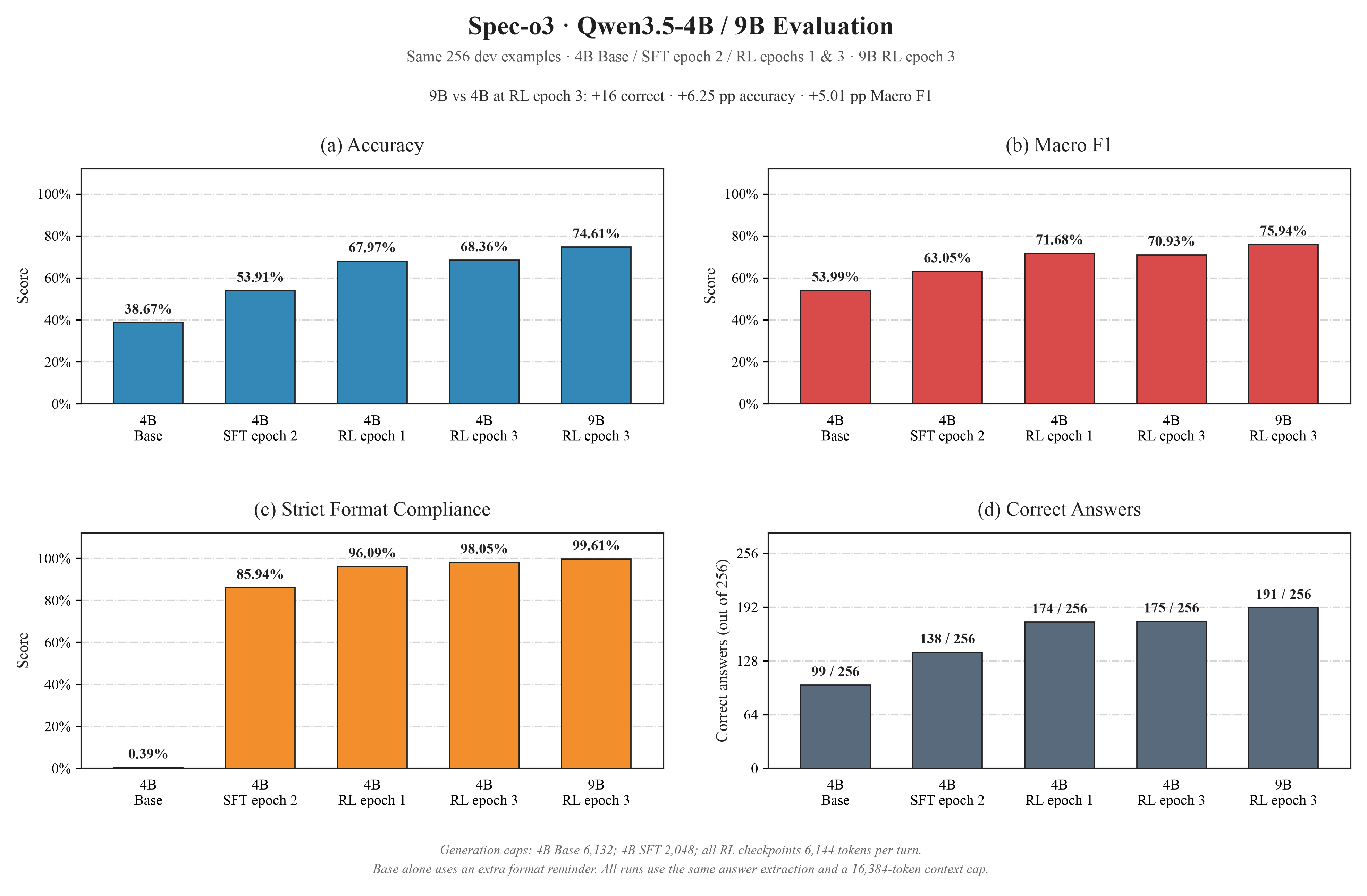
For 4B, SFT answers 39 more questions correctly than Base; the first RL run adds another 36. The new 4B RL epoch-3 checkpoint answers 1 more correctly than epoch 1 and reaches 98.05% format compliance, while Macro F1 declines slightly from 71.68% to 70.93%. More epochs did not improve every metric in this development evaluation.

The 9B RL epoch-3 checkpoint answers 191 / 256 correctly, 16 more than 4B RL epoch 3. Its accuracy is 6.25 percentage points higher and Macro F1 5.01 percentage points higher. Format compliance is 255 / 256 (99.61%), and all 1,011 tool calls execute successfully. For 4B RL epoch 3, these figures are 251 / 256 (98.05%) and 1,087 successful tool calls.

Per-task F1 for the epoch-3 checkpoints follows; parentheses show task sample counts:

Model	CC: carbon stars (56)	CV: cataclysmic variables (50)	GM: M-type giants (51)	SS: S-type stars (50)	WD: white dwarfs (49)
Qwen3.5-4B RL epoch 3	52.31%	61.11%	92.06%	79.17%	70.00%
Qwen3.5-9B RL epoch 3	67.80%	71.79%	87.72%	84.62%	67.80%

9B has higher F1 on CC, CV and SS, while 4B has higher F1 on GM and WD. The current 9B checkpoint has the best overall score, with differences across individual tasks.

The base model already answers some questions correctly, but follows the format inconsistently. That is a main focus of cold-start SFT in this experiment.

1. What does Spec-o3 actually do?

Here, “finding stars” means checking whether the spectrum of an existing candidate matches a target category. The model sees a curve with wavelength on the horizontal axis and flux on the vertical axis. Peaks, troughs and overall shape at different wavelengths provide classification evidence.

Spec-o3 focuses on candidate vetting in large spectroscopic surveys: automatically selected candidates still require inspection of ambiguous spectra. The paper organizes this into five independent YES/NO tasks. The table also lists the abbreviations used by our local data. Paper §3–4

Local task	Target category	Question
cv	Cataclysmic variables	Does this candidate show the spectral characteristics of a cataclysmic variable?
cc	Carbon stars	Is this candidate a carbon star?
ss	S-type stars	Is this candidate an S-type star?
gm	M-type giants	Is this candidate an M-type giant?
wd	White dwarfs	Is this candidate a white dwarf?

Each example asks about only one category. The input includes diagnostic guidance, such as relevant spectral lines and potentially confusing shapes. The model must connect that guidance with the image. Reference YES/NO labels remain in grading fields and do not enter the rollout input.

For example, local CV prompts mention Hα and Hβ. The model can inspect the full spectrum, request 6400–6700 Å, then inspect another band. It finally returns an answer in this structure, with the explanation inside the tags:

<answer>\boxed{YES}这里写基于光谱观察得到的解释。</answer>

The interesting part is that the model's current judgment determines which image it sees next.

2. Interleaved multimodal reasoning: thought alternates with new images

Spec-o3 calls this iMCoT, or Interleaved Multimodal Chain-of-Thought. A complete trajectory contains several reasoning segments, interspersed with new images returned by tools.

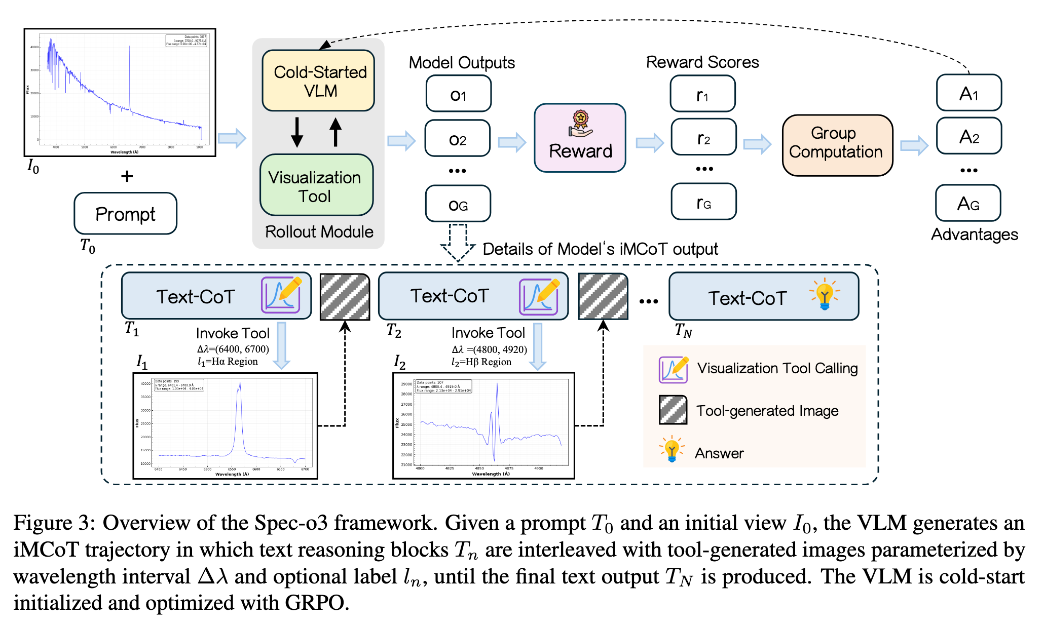
Source: Figure 3 of the Spec-o3 paper. The top shows group sampling, rewards and advantages. The bottom expands a trajectory alternating between textual reasoning and local spectrum plots.

Our implementation follows this interaction sequence:

用户问题 + 完整光谱图
→ assistant 思考，选择需要检查的波段
→ assistant 输出工具调用
→ 本地工具从光谱数组生成局部 PNG
→ tool observation 携带图片回到上下文
→ assistant 继续思考，再调用工具或输出最终答案

Training has two stages. Cold-start SFT uses complete demonstrations of observation, tool use and answering. GRPO then lets the model interact on training examples and receive rewards for its final answer and format. The authors' public implementation uses LLaMA-Factory for SFT and VeRL for RL; this chapter connects the process to PyTRIO. Authors' training guide

The original paper uses Qwen2.5-VL-3B/7B-Instruct. We use Qwen3.5-4B and Qwen3.5-9B with LoRA rank 32, so this is a transfer of the method to different base models and a different training stack. The focus is how the interaction and training pipeline works and what we actually measured.

Quick start: run SFT first

After installing UV, you can run the following commands. On first use, follow the terminal prompts to log in to PyTRIO and SwanLab:

git clone https://github.com/KMnO4-zx/agentic-rl-lab.git
cd agentic-rl-lab/09-spec-o3
uv sync --locked

uv run trio login
uv run swanlab login

uv run python prepare_data.py sft
uv run python train_sft.py --epochs 2

This downloads SFT data and images into datasets/sft/ and starts 2 epochs of cold-start training with the default Qwen3.5-4B LoRA configuration. At each epoch end, the terminal prints state_path for continued training and sampler_path for inference and evaluation.

The following sections explain the implementation. Data splits, full training parameters, the transition to RL, evaluation and plotting commands appear in Section 8: Running this experiment.

3. How do images and tool calls enter PyTRIO?

3.1 What changes in Qwen3.5's native template?

Qwen3.5's native template already supports thinking, tool calls and images, and preserves reasoning within the same tool-interaction chain. Starting from a pinned official template, we created qwen3_5_spec_o3.jinja with two main changes:

• Always preserve each assistant turn's reasoning_content, including earlier reasoning across new user questions, for full-trajectory supervision.
• Mark assistant learning spans with {% generation %} so the tokenizer returns the corresponding supervision mask.

Native role headers, visual markers and XML tool syntax remain. This format illustration shows one assistant turn moving from reasoning to a tool call:

<think>
下一步检查 Hα 附近的局部光谱。
</think>
<tool_call>
<function=spectral_visualization_tool>
<parameter=wavelength_range>
[6400, 6700]
</parameter>
<parameter=label>
Hα region
</parameter>
</function>
</tool_call>

After tool execution, its image enters the message corresponding to <tool_response>, and the next generation resumes from the assistant's <think> prefix. The template defines the message arrangement; SFT teaches what to generate at those positions.

3.2 Images enter the context through ImageChunk

protocol.py renders messages, then replaces every <|image_pad|> with a real image chunk. Text, images and following text retain their original order. This excerpt shows the structure, omitting encoding details:

prompt = trio.ModelInput(
    chunks=[
        trio.types.EncodedTextChunk(tokens=before_image_tokens),
        trio.ImageChunk(
            data=image_bytes,
            format="png",
            expected_tokens=image_tokens,
        ),
        trio.types.EncodedTextChunk(tokens=after_image_tokens),
    ],
)

data contains PNG bytes; file paths are used only for local reading. The matching base model's image processor computes expected_tokens from image dimensions, determining how many visual positions the image occupies. Second and third images returned by tools are appended the same way. PyTRIO multimodal guide

This length determines training alignment. Every image position enters the context, but receives zero training weight. Then target_tokens, masks and related arrays receive the autoregressive shift so that each position predicts the next token.

3.3 Where does the spectrum-zoom tool get its data?

The tool uses numerical spectra included in the public Parquet files. prepare_data.py extracts them into datasets/rl/spectra/*.npz, storing wavelength, flux and redshift. Initial images are saved separately in datasets/rl/images/.

The core calculation in tools.py is short:

wavelength = np.asarray(wavelength) / (1 + redshift)
low, high = wavelength_range
selected = (wavelength >= low) & (wavelength <= high)
ax.plot(wavelength[selected], flux[selected])

It corrects for redshift, selects the requested wavelength interval and redraws a PNG. Axes and display ranges change with the window, helping the model inspect local structure. If too few data points fall within the window, the tool returns a text explanation and the model continues in the next turn.

The dataset's .fits.gz names identify the original spectrum sources. This chapter's tool reads the prepared .npz files directly and returns a newly rendered spectrum plot plus a wavelength-range description.

4. Start with SFT to learn the complete interaction

4.1 SFT learns from full trajectories

Cold-start data already contains reasoning, tool calls, image observations and final answers. The authors used diagnostic guides and labels to help GPT-5 draft trajectories, which astronomy experts then revised and reviewed for SFT. Paper §3.2

The pinned dataset contains 942 trajectories, split by spectral object into 848 training and 94 validation examples. Training reads sft_train.jsonl. train_sharegpt.json preserves the original data, while sft_stats.json and sft_cleaning.jsonl record statistics and cleaning.

Some scientific symbols in the public text are corrupted. The script repairs encodings when the intended symbol is clear and keeps unresolved characters as visible markers. There are still 273 trajectories with such markers, and this training run retains them. This is a data-quality limitation; further experiments should review those positions.

For full-trajectory SFT, supervision covers:

Content	Included in SFT loss?
Assistant reasoning, tool calls, final answers and end tokens	Yes
System/user content and role headers	No
Text and images returned by tools	No

The model learns to generate the next reasoning segment and action from prior observations. Tool images remain visible and affect later predictions, while training targets focus on assistant-generated tokens.

4.2 Cold-start SFT

Before RL, SFT teaches Qwen3.5-4B the interleaved reasoning and tool-call format. The model reasons, emits a valid tool call when further inspection is needed, examines the returned local spectrum and continues until it answers.

Complete demonstrations connect these steps: analysis inside <think>, tool and wavelength parameters inside <tool_call>, another reasoning turn after the tool observation, and a conclusion with explanation inside <answer>. SFT supervises each assistant turn, preparing the model to organize its actions under the protocol before multi-turn GRPO exploration.

train_sft.py runs asynchronously with cross_entropy, supervising only assistant-generated content. The original 4B SFT run uses batch size 4, learning rate 2e-5, LoRA rank 32 and 2 epochs, totaling 424 training steps. Each epoch ends with validation loss and saved weights for further training and evaluation.

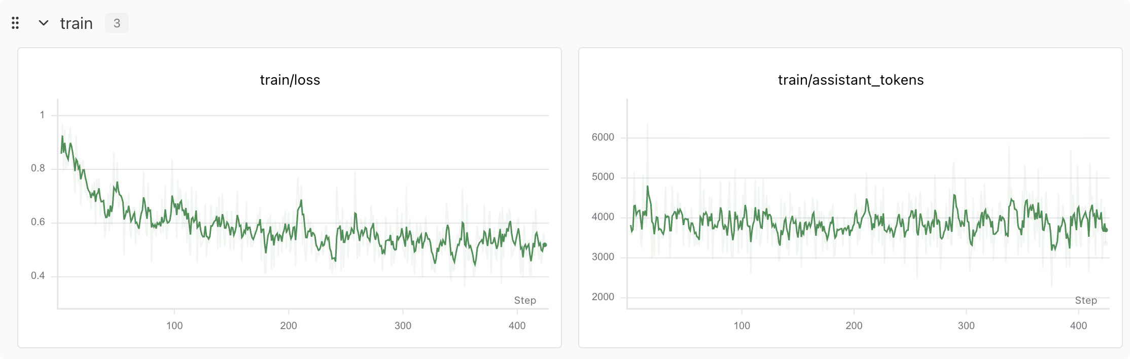
Full curves and configurations are public in the SFT records on the SwanLab experiment list.

Smoothed training loss falls from about 0.9 to about 0.5. The SFT checkpoint answers 138 / 256 development questions correctly and reaches 85.94% strict format compliance. We then add GRPO to improve wavelength selection and classification through actual tool interaction and final rewards.

5. Continue with GRPO to learn through interaction

5.1 Sample 8 complete tool trajectories per question

RL uses 3,108 questions from datasets/rl/bench_rl_train.jsonl. A batch takes 8 questions and generates 8 trajectories each, normally producing 64 rollouts.

The first-turn input is identical within a question, so one request can produce 8 beginnings:

first_turn = await sampler.sample_async(
    prompt=prompt,
    num_samples=args.group_size,
    sampling_params=sampling_params,
)

Later, trajectories may select different wavelength bands and receive different images. Each therefore continues with its own context and num_samples=1. The question retains its 8 branches, and finished branches stop requesting generations. Questions and branches run concurrently through asyncio.gather().

The batch shares one sampler version. Model updates begin only after all rollouts finish, and the next batch creates a sampler from the updated weights. Rewards and saved old log probabilities within the group therefore correspond to one policy version.

An epoch generates 3,108 × 8 = 24,864 trajectories across 389 rollout batches. The last batch has 4 questions and 32 trajectories. The outer terminal progress bar counts trajectories; the inner bar tracks the current batch. Actual optimizer updates can be fewer if an entire batch lacks a relative training signal.

5.2 Rewards depend only on answers and format

The reward is:

$$r(\tau )=\mathbb{1}[\text{correct answer}]-0.2\mathbb{1}[\text{invalid format}]$$

Answer	Format	Reward
Correct	Valid	1.0
Correct	Invalid	0.8
Incorrect	Valid	0.0
Incorrect	Invalid	-0.2

There is no additional reward for the number of tool calls. Whether another image is useful must be learned through the final task result.

Training reward extraction reads YES/NO at the beginning of the final turn's body after reasoning ends, allowing partially missing tags to receive correctness credit. Evaluation instead extracts the last complete answer block after the final </think> in the last turn. These are separate implementations.

5.3 Relative learning requires differences within a group

Rewards from the 8 trajectories for a question determine their advantages:

$$A_i=\frac{r_i-\mathrm{mean}(r_1,\dots ,r_8)}{\mathrm{std}(r_1,\dots ,r_8)+{10}^{-6}}$$

The standard deviation is the sample standard deviation, ddof=1. Even an incorrect answer receiving 0 has negative advantage if other trajectories in the group receive higher rewards.

A group is skipped only when all rewards are identical. Because format affects reward, an all-correct group can still provide a signal if formats differ. Skipped groups remain in training statistics. The current code does not resample to refill informative groups.

5.4 Update only the assistant tokens actually generated

rollout.py retains the tokens and log probabilities returned by the service for every turn. Continuation preserves the generated history and encodes only the new tool observation and next prefix, avoiding token changes caused by rerendering assistant text.

Assistant tokens in a trajectory share its advantage. Questions, images, tool observations and program-inserted separators are context only, with zero advantage. The batch of Datums then uses PyTRIO's built-in ppo loss with clipping bounds [0.8, 1.2] and one update per batch.

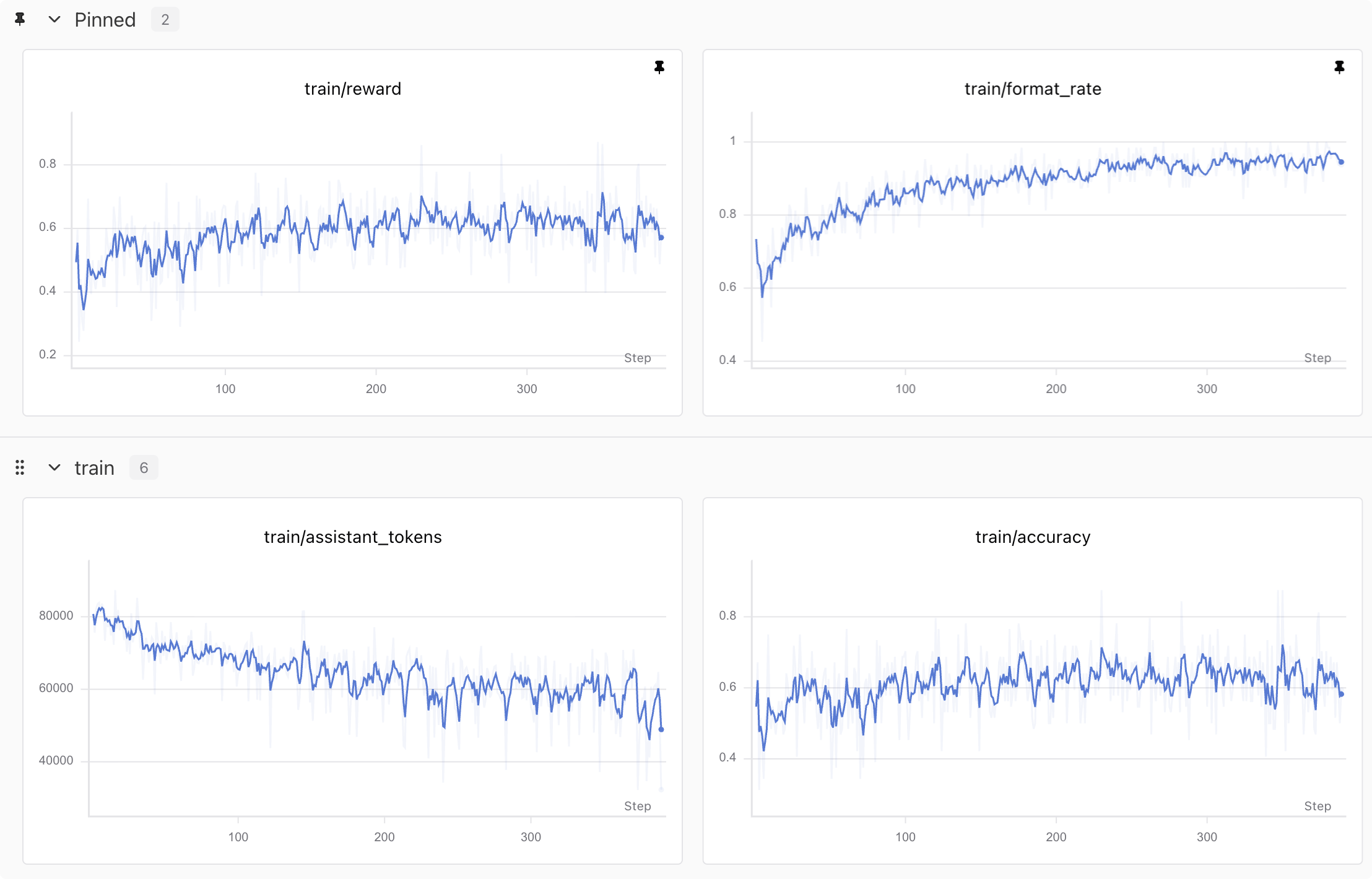
This figure preserves the original 4B RL epoch-1 training run. New independent 4B and 9B epoch-3 evaluations appear in Section 0. Full RL curves and configurations are also on the public SwanLab experiment list.

Format compliance rises clearly, approaching 0.95 later in training. Reward and training accuracy improve with fluctuations and do not rise monotonically throughout the second half. Each step sees different questions, so these curves describe training behavior; final performance still comes from the fixed development evaluation.

The lower-left train/assistant_tokens is the total token count across the current batch's effective training examples. It changes with trajectory lengths, skipped equal-reward groups and final-batch size. To assess whether average reasoning becomes shorter, inspect per-trajectory lengths or rollout/mean_generated_tokens.

6. Why does cold-start SFT matter?

Base makes some correct judgments but has only 0.39% strict format compliance. After SFT, that reaches 85.94%. The change shows how full-trajectory demonstrations help this model follow the interaction protocol.

SFT teaches the interleaved structure reasoning → tool call → image observation → further reasoning → final answer: specifying valid tool arguments, analyzing new images and ending responses correctly. Together these abilities produce an executable multi-turn trajectory.

With that cold start, GRPO can optimize wavelength selection and classification through final rewards within an interaction process the model already knows.

7. What PyTRIO contributes to the research workflow

The original paper trains with 8 NVIDIA H100 GPUs. Paper §4.2 Obtaining compute, deploying multi-GPU training and connecting training with inference take effort. Here I used PyTRIO to run Qwen3.5-4B LoRA SFT, tool interaction and GRPO, leaving model computation and weight storage to the remote service.

The practical benefits during this experiment were:

• Starting an idea sooner. With data and a Python loop ready, computation can be submitted through the API. The local machine renders spectra, organizes messages and computes rewards. The service executes multi-GPU training, so an ordinary CPU machine can drive the experiment. PyTRIO introduction
• Organizing parallel comparisons. Different learning rates, rewards or seeds can use separate training jobs with independent LoRA weights and optimizer states, while the service schedules shared compute. Experiments need not be tied to one GPU server. Multi-job scheduling
• Keeping attention on research questions. I mainly worked on interleaved reasoning, image/text inputs, tool observations, rewards and evaluation rules. Changes to those parts still use the same training APIs, checkpoints and SwanLab records.

The original 4B usage record follows. Its SFT and RL epoch-1 training sessions total ¥699.68, excluding evaluation and debugging sessions. This amount covers only the two historical training sessions shown, not the new 4B/9B epoch-3 training or evaluation.

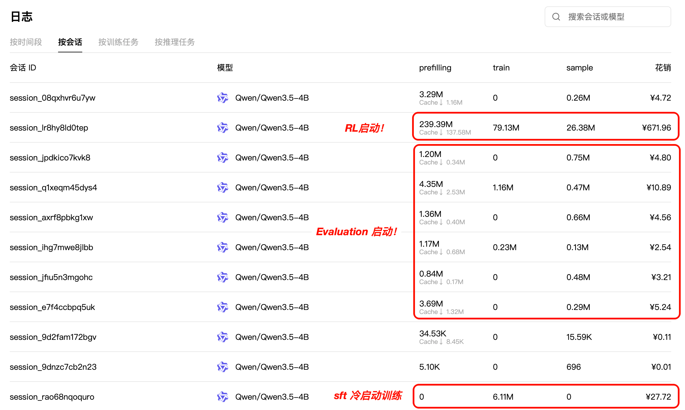
The two labeled training sessions are listed below. M means one million tokens:

Session	Prefilling	Train	Sample	Cost
Cold-start SFT	0	6.11M	0	¥27.72
4B RL epoch 1	239.39M	79.13M	26.38M	¥671.96
Total for these two training sessions				¥699.68

The original 4B experiment took me less than one day from reading the paper to completion.

For me, PyTRIO shortened the path from wanting to try a method to having results to analyze. That makes it easier to run an idea, add controls, inspect failed trajectories and adjust training iteratively.

8. Running this experiment

8.1 Install the environment and log in

With UV installed, clone the project and install its locked dependencies:

git clone https://github.com/KMnO4-zx/agentic-rl-lab.git
cd agentic-rl-lab
uv sync --locked
cd 09-spec-o3

uv run trio login
uv run swanlab login

In an existing checkout, run uv sync --locked from the root, then enter 09-spec-o3/. All commands below run in that directory. The project uses Python 3.13+ and PyTRIO 0.2.9. Local code handles data, plotting and orchestration; the remote service handles model training and sampling. Training uses authentication saved by the CLI.

8.2 Prepare SFT data before RL data

uv run python prepare_data.py sft
uv run python prepare_data.py bench

The order matters: bench reads the SFT object list to keep spectra seen in SFT out of dev. Downloads, images and processed files are stored as follows:

datasets/
├── sft/
│   ├── train_sharegpt.json
│   ├── images/
│   ├── sft_train.jsonl       # 848 条，用于 SFT
│   ├── sft_val.jsonl         # 94 条，用于验证 loss
│   ├── sft_cleaning.jsonl
│   └── sft_stats.json
└── rl/
    ├── data/                 # 下载的原始 Parquet
    ├── images/               # 初始光谱图片
    ├── spectra/              # 工具使用的 NPZ 数组
    ├── bench_rl_train.jsonl  # 3,108 条，用于 RL
    ├── bench_dev.jsonl       # 256 条，本章评测集
    ├── bench_test.jsonl      # 6,754 条，尚未评测
    └── bench_stats.json

The script downloads pinned dataset revisions into these directories. The current configuration uses Hugging Face's official HTTP channel with Xet disabled; reruns reuse completed files. JSONL stores absolute image and spectrum paths, so moving the directory or machine requires preparing the data again to update them.

8.3 Run 2 epochs of SFT

uv run python train_sft.py \
    --base-model Qwen/Qwen3.5-4B \
    --epochs 2 \
    --batch-size 4 \
    --rank 32 \
    --learning-rate 2e-5 \
    --run-name spec-o3-sft \
    --swanlab-mode online

The script defaults to 1 epoch, so the command explicitly passes --epochs 2. --model-revision defaults to main, as in the recorded SFT run. To pin tokenizer and image-processor files, use the revision from this chapter's data preparation and evaluation: 851bf6e806efd8d0a36b00ddf55e13ccb7b8cd0a.

For 9B, change --base-model to Qwen/Qwen3.5-9B and use a separate --run-name. A pinned revision must belong to the corresponding model repository; the commit above is only for 4B.

Keep the epoch-2 state_path and sampler_path after training. They are used for subsequent RL and SFT evaluation, respectively.

8.4 Continue RL from the SFT state

Replace the placeholder below with the state_path printed by training or obtained from the PyTRIO weights console:

uv run python train_rl.py \
    --state-path '<SFT epoch 2 的 state_path>' \
    --epochs 1 \
    --batch-size 8 \
    --group-size 8 \
    --learning-rate 1e-6 \
    --max-turns 8 \
    --max-tokens 2048 \
    --max-seq-len 16384 \
    --save-every 100 \
    --run-name spec-o3-rl \
    --swanlab-mode online

--max-tokens limits each generation; --max-seq-len limits total context including text, images and tool history. --max-turns 8 allows at most 8 assistant generations, including the final answer. The current implementation executes tool calls only during the first 7 turns.

The command preserves the original 1-epoch 4B run. For 3 epochs from the SFT state, set --epochs 3. For 9B, supply its SFT state_path; the script restores the corresponding base model from the checkpoint. Use separate --run-name values for separate experiments.

The current script saves state and sampler weights every 100 cumulative rollout steps and at epoch ends. Periodic saving was added after the original RL experiment to retain intermediate weights in later runs. Logs distinguish rollout steps from actual updates, which differ when an entire batch is skipped.

The main differences between the authors' public configuration and the original 4B run are:

Item	Authors' public configuration	Original 4B experiment
Base model	Qwen2.5-VL-3B/7B-Instruct	Qwen3.5-4B
Parameter updates	SFT updates all language-model parameters and freezes vision components	LoRA rank 32
SFT / RL epoch	5 / 3	2 / 1
SFT / RL learning rate	2e-5 / 1e-6	2e-5 / 1e-6
SFT schedule	Cosine, warmup ratio 0.05	Constant learning rate
RL questions per batch / trajectories per question	64 / 8	8 / 8
Sequence budget	SFT cutoff 32,768; RL max response 32,768	Training trajectories use a total context budget of 16,384

The authors' settings come from pinned SFT YAML and RL YAML files. This chapter also does not reproduce every upstream loss detail. The results describe our method transfer and cannot be directly aligned with the paper's benchmark scores.

8.5 Evaluate 4B Base, SFT and 4B / 9B RL

The commands retain the generation budgets used in the opening table. Replace each placeholder with its corresponding sampler_path:

# Base：不传 model-path，脚本自动追加格式提醒。
uv run python eval.py \
    --base-model Qwen/Qwen3.5-4B \
    --output outputs/base-dev \
    --max-tokens 6132 \
    --max-seq-len 16384

# SFT epoch 2。
uv run python eval.py \
    --base-model Qwen/Qwen3.5-4B \
    --model-path '<SFT epoch 2 的 sampler_path>' \
    --output outputs/sft-dev \
    --max-tokens 2048 \
    --max-seq-len 16384

# SFT → RL epoch 1。
uv run python eval.py \
    --base-model Qwen/Qwen3.5-4B \
    --model-path '<RL epoch 1 的 sampler_path>' \
    --output outputs/sft-rl \
    --max-tokens 6144 \
    --max-seq-len 16384

# 4B RL epoch 3。
uv run python eval.py \
    --base-model Qwen/Qwen3.5-4B \
    --model-path '<4B RL epoch 3 的 sampler_path>' \
    --output outputs/rl-4b-e3 \
    --max-tokens 6144 \
    --max-seq-len 16384

# 9B RL epoch 3。
uv run python eval.py \
    --base-model Qwen/Qwen3.5-9B \
    --model-path '<9B RL epoch 3 的 sampler_path>' \
    --output outputs/rl-9b-e3 \
    --max-tokens 6144 \
    --max-seq-len 16384

--output names the evaluation artifact directory, containing metrics.json, per-example trajectories.jsonl and tool-generated images. Use a new directory for a new evaluation to preserve prior records. Defaults are bench_dev.jsonl, concurrency 16, temperature 0.6, seed 42 and at most 8 turns.

--base-model must match the sampler weights' base model. The tokenizer, image processor and sampling client all use that model. --model-revision selects its Hugging Face file revision; by default, 4B uses the pinned revision and 9B uses main.

The Base and SFT table values come from metrics-reparsed.json, computed by rescoring existing trajectories. RL values come from metrics.json under the new extraction rules. The current eval.py already includes those rules and writes new results directly to metrics.json.

To compare SFT and RL with matched generation budgets, run the following next:

uv run python eval.py \
    --base-model Qwen/Qwen3.5-4B \
    --model-path '<SFT epoch 2 的 sampler_path>' \
    --output outputs/sft-dev-6144 \
    --max-tokens 6144 \
    --max-seq-len 16384

This matched-budget reevaluation remains pending; its results are not in this article's table.

8.6 Plotting and code-reading order

uv run python analysis.py

The script plots this article's five fixed results into images/results_comparison.png and exports a matching vector PDF. Its four panels compare accuracy, Macro F1, strict format compliance and correct answers, labeling model size and training stage. It does not read new evaluation directories; update the script's data and captions after obtaining new results.

Read the code from data preparation through input construction, interaction and training:

File	Responsibility
prepare_data.py	Download, clean and split data; save images and spectrum arrays
templates/qwen3_5_spec_o3.jinja	Render multi-turn image/text messages and mark assistant supervision spans
protocol.py	Build image chunks and SFT/RL Datums; parse actions
tools.py	Redraw a local spectrum for a wavelength interval
rollout.py	Execute a complete tool trajectory and retain actual tokens and log probabilities
train_sft.py	Asynchronous SFT, validation and state/sampler saving
train_rl.py	Group sampling, rewards, advantages, PPO updates and checkpoints
eval.py	Independent evaluation with classification metrics, trajectories and tool images
analysis.py	Plot this article's fixed results